Cormack-Jolly-Seber Models
Cormack-Jolly-Seber Models (CJS) are a relatively old model type that has been long used in the field of wildlife biology. This model type uses a detection history (or, as its also called, a capture history) to estimate detection probability for marked individuals and, thereby, estimate "apparent" survival. I have NOT written a full tutorial for this model type yet, however, I will paste my R code below along with a set of fake data.
Fake dataset can be downloaded here:
| ||||
...and the R script is pasted here; check back in soon for a detailed update to this page and, remember, email me with questions. Oh, and a quick thing about data formatting:
#####################################################################################################
# a few notes about importing data into RMark. Hands-down, the greatest challenge associated with
# data management for RMark is importing your detection history (e.g., "0010110") without losing
# the leading zeros to formatting (e.g., Excel and R like to convert that string to a numeric = 10,110).
# The best way I have found to do this is by creating your detection history in individual columns (one
# column for each visit), and then using =CONCATENATE to bring everything together into one cell. Then
# re-paste the contents of these cells (paste values) into the first column but change the cell format
# to text. Save this file as a regular excel file for your records but then copy ALL of the data for
# analysis into notepad and save as a .txt - this will be ideal for analysis and these steps are all
# omitted from the analysis below. Once I get a change to design this web page in earnest, I will add more
# of these details. Feel free to email me if you have questions!
#####################################################################################################
#####################################################################################################
# a few notes about importing data into RMark. Hands-down, the greatest challenge associated with
# data management for RMark is importing your detection history (e.g., "0010110") without losing
# the leading zeros to formatting (e.g., Excel and R like to convert that string to a numeric = 10,110).
# The best way I have found to do this is by creating your detection history in individual columns (one
# column for each visit), and then using =CONCATENATE to bring everything together into one cell. Then
# re-paste the contents of these cells (paste values) into the first column but change the cell format
# to text. Save this file as a regular excel file for your records but then copy ALL of the data for
# analysis into notepad and save as a .txt - this will be ideal for analysis and these steps are all
# omitted from the analysis below. Once I get a change to design this web page in earnest, I will add more
# of these details. Feel free to email me if you have questions!
#####################################################################################################
# Another little note: RMark doesn't like covariate names longer than 10
# characters for some reason
#########################################################
# /\ /\ /\ /\
# p q p q p q p q
# _\| \ / |/_ _\| \ / |/_ _\| \ / |/_ _\| \ / |/_
# \// \\/ \// \\/ \// \\/ \// \\/
# `| |` `| |` `| |` `| |`
# | | ,/_ | | ,/_ | | ,/_ | | ,/_
# _\, | |//\ _\, | |//\ _\, | |//\ _\, | |//\
# /\\| ;/ /\\| ;/ /\\| ;/ /\\| ;/
# \; \ \; \ \; \ \; \
# '. \ '. \ '. \ '. \
# .-. \ | .-. \ | .-. \ | .-. \ |
#` '.__// ` '.__// ` '.__// ` '.__//
# `"` `"` `"` `"`
#########################################################
# install.packages("RMark") # download if needed
library(RMark)
setwd("C:\\Users\\DJ\\Desktop\\rmark practice")
salamanders=import.chdata("salamanders.txt", field.types=c("f","n","n","n","n"))
# note, it automatically knows that ch = character so you do not need to specify it.
# alternatively:
# salamanders<-read.table("salamanders.txt", header=TRUE, colClasses=c("character", "factor", "numeric", "numeric", "numeric", "numeric"))
summary(salamanders)
salamanders.processed=process.data(salamanders,groups=("sex")) # define a group
salamanders.ddl=make.design.data(salamanders.processed) # design data relate parameters to time, age, cohort and group structure.
######################################
# Creating Cormack-Jolly-Seber Models
######################################
phidot.pdot = mark(data = salamanders.processed, ddl = salamanders.ddl, model = "CJS",
model.parameters = list(Phi=list(formula=~1), p=list(formula=~1)))
phidot.psex = mark(data = salamanders.processed, ddl = salamanders.ddl, model = "CJS",
model.parameters = list(Phi=list(formula=~1), p=list(formula=~sex)))
phidot.pphenotype = mark(data = salamanders.processed, ddl = salamanders.ddl, model = "CJS",
model.parameters = list(Phi=list(formula=~1), p=list(formula=~pheno_gray+pheno_rain)))
phisex.pdot = mark(data = salamanders.processed, ddl = salamanders.ddl, model = "CJS",
model.parameters = list(Phi=list(formula=~sex), p=list(formula=~1)))
phiphenotype.pdot = mark(data = salamanders.processed, ddl = salamanders.ddl, model = "CJS",
model.parameters = list(Phi=list(formula=~pheno_gray+pheno_rain), p=list(formula=~1)))
phimass.pdot = mark(data = salamanders.processed, ddl = salamanders.ddl, model = "CJS",
model.parameters = list(Phi=list(formula=~mass), p=list(formula=~1)))
philength.pdot = mark(data = salamanders.processed, ddl = salamanders.ddl, model = "CJS",
model.parameters = list(Phi=list(formula=~length), p=list(formula=~1)))
######################################
# Ranking candidate model set
######################################
salamander.table <- collect.models(type = "CJS")
salamander.table
## Exploring individual models can be done using <model>$results; for example:
philength.pdot$results
#######################################
# Making and Graphing Model Predictions
#######################################
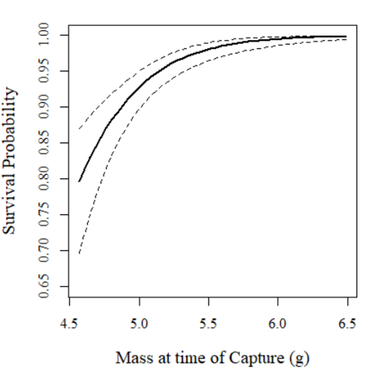
phi.mass.predictions = covariate.predictions(model = phimass.pdot, data = data.frame(index=rep(1,50),
mass=seq(from=min(salamanders$mass), to=max(salamanders$mass), length.out = 50)))
# graphing model predictions
with(phi.mass.predictions$estimates,
{
plot(mass, estimate,type="l",lwd=2,xlab="Mass at time of Capture (g)",
ylab="Survival Probability",ylim=c(0.65,1),family="serif", cex.lab=1.25)
lines(mass,lcl,lty=2)
lines(mass,ucl,lty=2)
})
cleanup(ask=FALSE) # this deletes all the pesky MARK files