Multi-season Occupancy Models
The 'big brother' of the single-season occupancy model, the multi-season occupancy model (aka 'dynamic occupancy model') is useful for modeling and making predictions over multiple years. Although it might seem tempting to treat data from different seasons separately using individual sets of single-season occupancy models, the benefit of using multi-season occupancy models is that they allow the estimation of two additional parameters: colonization ('gamma') and extinction ('epsilon'). Like the single-season occupancy model, we also have our familiar parameters: occupancy ('psi') and detection ('p')... with one caveat: with this model type, one of these four parameters must be derived; that is, you can only obtain the parameter estimate for the first season of the study and patterns thereafter must be inferred. Because the parameters of interest in multi-season occupancy models are frequently gamma and epsilon, psi is typically the derived parameter. What this means is that, when we estimate 'psi' or 'occupancy', it should be thought of as 'first season's occupancy'. Consecutive season's occupancy must be inferred from colonization and extinction. Here I walk you through a simple example of a multi-season occupancy analysis using some fake data for a fake organism in fake habitat. Begin by downloading the dataset:
|
| |||||
Let's begin by loading the needed packages (unmarked and AICcmodavg):
library(unmarked)
library(AICcmodavg)
Next, of course, you will want to set your working directory ('setwd') and import the .csv ('read.csv'). You can set your working directory easily by copying the address of your file location from your file explorer, pasting it into R, and then replacing the single slashes (\) with double slashes (\\):
setwd("C:\\Users\\DJ\\Desktop")
data1<-read.csv("colext_data_practice.csv", header=TRUE)
Next, it's useful to define some of your input datasets. To accomplish this, it helps to define the number of sites (M), the number of secondary sampling periods (J; i.e., number of visits/season) and the number of primary sampling periods (T; i.e., the number of seasons). The first three lines of codes accomplish this. Using these pieces, it's a bit easier to define the input data which, for this dataset include our detection histories:
Note that, unlike single-season models, all inputs for multi-season occupancy models are matrices. The arguments for a matrix are:
matrix(data, nrow, ncol)
yy: The detection history should be ncol = J x T representing your surveys
time, date: These detection covariates should be ncol = J x T because you resample during every sampling occasion
thistle, dist: These site covariates should be a single column each - one value for each site.
year: This yearly site covariate changes every season. It should be one value for each primary sampling period.
M <- (nrow(data1)) # Number of sites = m
J <- 2 # Number secondary sample periods
T <- 3 # Number primary sample periods
# matrix(data, nrow, ncol)
yy <- matrix(c(data1$det1.1, data1$det1.2, data1$det2.1, data1$det2.2, data1$det3.1, data1$det3.2), M, J*T) # make a matrix of the input data (detection histories across all years)
time <- matrix(c(data1$time1.1, data1$time1.2, data1$time2.1, data1$time2.2, data1$time3.1, data1$time3.2), M, J*T)
date <- matrix(c(data1$date1.1, data1$date1.2, data1$date2.1, data1$date2.2, data1$date3.1, data1$date3.2), M, J*T)
thistle<- matrix(c(data1$thistle), nrow(data1), 1, byrow=TRUE)
dist<- matrix(c(data1$dist), nrow(data1), 1, byrow=TRUE)
year <- matrix(c('1','2','3'), nrow(data1), T, byrow=TRUE)
Now that the data are all 'organized' into parts, we must create an 'unmarked frame'. This data object is that used by unmarked for analysis. Note that the unmarked frame has four main parts:
1) "y" (the occupancy data; detection histories),
2) "yearlySiteCovs" (covariates which are site specific but change every year (e.g., vegetation succession)),
3) "siteCovs" (covariates which are site specific but remain stable over time (e.g., elevation)),
4) "obsCovs" (covariates which are observation-specific... like time since sunrise (tssr) and wind). These change during each visit to a single site. Note that we have two visits/season and three seasons so we therefore have six columns within "y" (each survey for the organism) and six columns for each of our "obsCovs" (e.g., wind during each survey) but only ONE for each of our "siteCovs"... these things remain the same during each survey (e.g., canopy cover doesn't change, no matter how many times you visit).
umf1 <- unmarkedMultFrame(y = yy,
yearlySiteCovs = list(year = year),
siteCovs= data.frame(thistle=thistle, dist=dist),
obsCovs = list(time = time, date = date), numPrimary=T)
Time to create some occupancy models! The model function ("occu") has three main arguments:
~"psi" (ψ), ~"gamma" (γ), ~"epsilon" (ε), ~"p", and "data". As mentioned above, ψ is first-season's occupancy. If you want to keep any parameter constant, place a 1 here. Colonization rate is γ and extinction rate is ε. As with other occupancy frameworks, detection probability is represented by p. "data" should be your unmarked frame. Below I create single-covariate occupancy models for detection probability but keep ψ, γ, and ε constant (we will get to them next). I also created a null model called "p.null" which includes no covariates for any parameter.
~"psi" (ψ), ~"gamma" (γ), ~"epsilon" (ε), ~"p", and "data". As mentioned above, ψ is first-season's occupancy. If you want to keep any parameter constant, place a 1 here. Colonization rate is γ and extinction rate is ε. As with other occupancy frameworks, detection probability is represented by p. "data" should be your unmarked frame. Below I create single-covariate occupancy models for detection probability but keep ψ, γ, and ε constant (we will get to them next). I also created a null model called "p.null" which includes no covariates for any parameter.
p.null <- colext(psiformula= ~1, gammaformula = ~ 1, epsilonformula = ~ 1, pformula = ~ 1, data = umf1, method="BFGS")
p.date <- colext(psiformula= ~1, gammaformula = ~ 1, epsilonformula = ~ 1, pformula = ~ date, data = umf1, method="BFGS")
p.time <- colext(psiformula= ~1, gammaformula = ~ 1, epsilonformula = ~ 1, pformula = ~ time, data = umf1, method="BFGS")
p.year <- colext(psiformula= ~1, gammaformula = ~ 1, epsilonformula = ~ 1, pformula = ~ year, data = umf1, method="BFGS")
Once those models are run, I usually create a list containing each model and then use the aictab() function to rank the models in descending order of AIC and create a table. This function is really quite handy.
modlist1<-list(p.null=p.null, p.date=p.date, p.time=p.time, p.year=p.year)
aictab(modlist1)
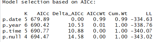
And here is the ranked model set:
|
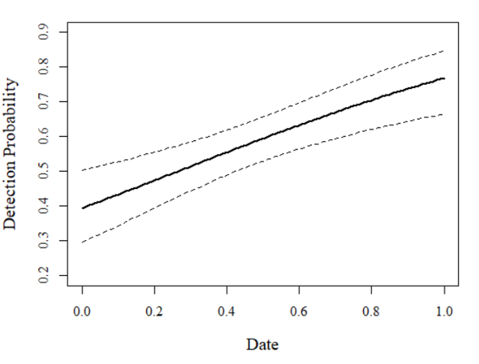
This result suggests that date might be a predictor of detection probability. The beta coefficient on the date parameter's 95% confidence intervals do not overlap (first line of code below shows this) and the null model is >2.0 from the date model suggesting that p.date is a better model. Let's visualize this pattern by predicting detection probability using the date model:
confint(p.date, type="det")
# Graphing detection over date
nd <- data.frame(("date"=(seq(0, 1, length.out = 100))))
colnames(nd)<-c("date")
pred.p <- predict(p.date, type='det', newdata=nd)
print(predictions<-cbind(pred.p, nd))
plot(1, xlim=c(0,1), ylim=c(0.2,0.9), type="n", axes=T, xlab="Date",
pch=20, ylab="Detection Probability", family="serif",
cex.lab=1.25, cex.main=1.75)
lines(predictions$date, predictions$Predicted, col="black", lwd=2)
lines(predictions$date, predictions$lower, lty=2, col="black")
lines(predictions$date, predictions$upper, lty=2, col="black")
|
This result suggests that, as date advances, detection probability for the focal species increases.
For the rest of this analysis, we will analyze with a covariate for date in the detection component of the model. This will account for the effect of date on detection probability and allow us to better ascertain habitat effects on the state variables of interest: occupancy, colonization, and extinction. Let's continue by modeling first-year occupancy (ψ). In particular, we create occupancy models using "date" to explain detection and one of our site covariates ("thistle") to explain occupancy - including a detection-only model ("psi.null") as our null model. We also create a list of models and rank them using the same function as above (aictab):
psi.null <- colext(psiformula= ~1, gammaformula = ~ 1, epsilonformula = ~ 1, pformula = ~ date, data = umf1, method="BFGS")
psi.thistle <- colext(psiformula= ~thistle, gammaformula = ~ 1, epsilonformula = ~ 1, pformula = ~ date, data = umf1, method="BFGS")
modlist2<-list(psi.null=psi.null, psi.thistle=psi.thistle)
aictab(modlist2)
|
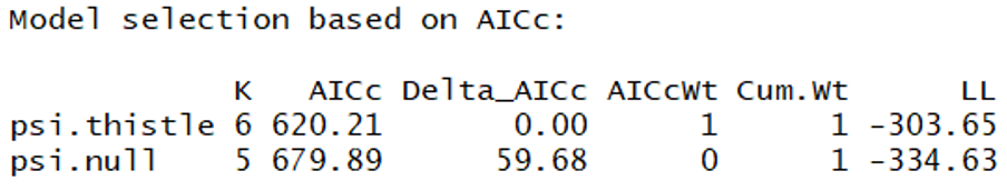
Based on this AIC table, it seems that thistle is an important predictor. The null model is > 2.0 from this model suggesting that it is not "competing" (in the words of Burnham and Anderson 2002). Let's check the confidence intervals on the beta coefficient for the thistle cover term in that psi.thistle model:
confint(psi.thistle, type="psi")
Non-overlapping with zero! That suggests the covariate is a strong predictor! Let's visualize this relationship using a graph of the predicted relationship based on that model and some 'fake data' (as we did with the detection example above):
nd2 <- data.frame(("thistle"=(seq(0, 100, length.out = 100))))
colnames(nd2)<-c("thistle")
pred.psi <- predict(psi.thistle, type='psi', newdata=nd2)
print(predictions<-cbind(pred.psi, nd2))
plot(1, xlim=c(0,100), ylim=c(0,1), type="n", axes=T, xlab="Thistle (% cover)",
pch=20, ylab="First-year Occupancy Probability", family="serif",
cex.lab=1.25, cex.main=1.75)
lines(predictions$thistle, predictions$Predicted, col="black", lwd=2)
lines(predictions$thistle, predictions$lower, lty=2, col="black")
lines(predictions$thistle, predictions$upper, lty=2, col="black")
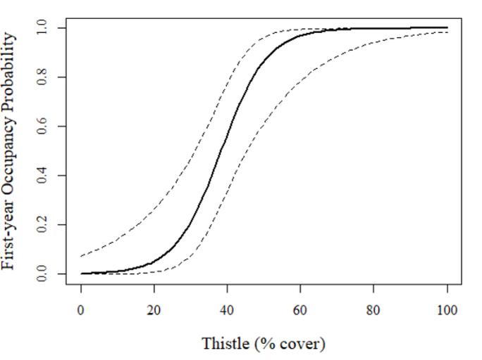
|
Very cool! In this case, there seems to be a sigmoidal relationship with thistle cover with the low-thistle sites having low occupancy (<0.10) and high thistle sites hosting very high occupancy (around 1.0).
Ok, this leaves us with our two 'new' parameters special to multi-season occupancy models: colonization (gamma; γ) and extinction (epsilon; ε). Let's model one of those here: colonization. We test this in a similar way to first-season occupancy, however, we know that our main covariate of interest (thistle) DOES impact first-year occupancy. Because occupancy models consider each parameter separately but we want to account for as much variation as possible, let's include thistle as a covariate for ψ (first season occupancy) and as a covariate for γ (colonization). Let's also keep our covariate for p (date) and test against a null model. As before, we create a list of covariates and use the aictab function on the list:
Ok, this leaves us with our two 'new' parameters special to multi-season occupancy models: colonization (gamma; γ) and extinction (epsilon; ε). Let's model one of those here: colonization. We test this in a similar way to first-season occupancy, however, we know that our main covariate of interest (thistle) DOES impact first-year occupancy. Because occupancy models consider each parameter separately but we want to account for as much variation as possible, let's include thistle as a covariate for ψ (first season occupancy) and as a covariate for γ (colonization). Let's also keep our covariate for p (date) and test against a null model. As before, we create a list of covariates and use the aictab function on the list:
gamma.null <- colext(psiformula= ~thistle, gammaformula = ~ 1, epsilonformula = ~ 1, pformula = ~ date, data = umf1, method="BFGS")
gamma.thistle <- colext(psiformula= ~thistle, gammaformula = ~ thistle, epsilonformula = ~ 1, pformula = ~ date, data = umf1, method="BFGS")
modlist3<-list(gamma.null=gamma.null, gamma.thistle=gamma.thistle)
aictab(modlist3)
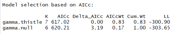
|
Let's now visualize the relationship:
nd3 <- data.frame(("thistle"=(seq(0, 100, length.out = 100))))
colnames(nd3)<-c("thistle")
pred.gam <- predict(gamma.thistle, type='col', newdata=nd3)
print(predictions<-cbind(pred.gam, nd3))
plot(1, xlim=c(0,100), ylim=c(0,1), type="n", axes=T, xlab="Thistle (% cover)",
pch=20, ylab="Colonization Probability", family="serif",
cex.lab=1.25, cex.main=1.75)
lines(predictions$thistle, predictions$Predicted, col="black", lwd=2)
lines(predictions$thistle, predictions$lower, lty=2, col="black")
lines(predictions$thistle, predictions$upper, lty=2, col="black")
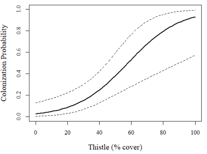
|
As with the post on single-season occupancy models, this post really just 'scratches the surface' of dynamic occupancy modeling. I hope to some day include more in-depth tutorials on dynamic occupancy models but this should 'get your feet wet' for those totally new to multi-season occupancy models in unmarked. Feel free to email me if you have any questions on the content of this tutorial and feel free to share with those interested!