Summary of Means
One of the most basic things one often needs to accomplish with new data is a simple data summary consisting of means (and associated error) plotted on a barplot. Although we all have our personal preference as to how such a plot should look, I provide here two functions to get this done.
The first is a data summary function. This function takes a few arguments and summarizes your data for you. Here's the code and example usage.
First the function itself:
The first is a data summary function. This function takes a few arguments and summarizes your data for you. Here's the code and example usage.
First the function itself:
library("dplyr")
library("rlang")
library("lazyeval")
ci <- function(x) {sqrt(sd(x)/length(x)) * 1.96}
summary_table <- function(data, groups, values) {
data %>%
group_by(!!sym(groups)) %>%
summarise("Mean" = mean(!!sym(values), na.rm = TRUE), "ConfInt" = ci(!!sym(values)))
}
Next, creating a fake dataset:
data1 <- data.frame(
"animal" = c(rep("mouse", 10), rep("chipmunk", 10), rep("squirrel", 10)),
"weight" = c(rnorm(10, mean = 10, sd = 1), rnorm(10, mean = 50, sd = 5),
rnorm(10, mean = 100, sd = 11))
)
summary(data1)
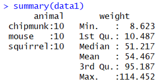
|
Now let's run the summary:
sum1 <- summary_table(data = data1, "animal", "weight")
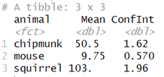
|
Great! A summary of the means for each category along with the 95% confidence interval
Boxplot with 95% CIs for Summary Table
Next, we might wish to depict this table in a graphical way, like a boxplot. The function below (called "basic_boxplot") can accomplish this. 95% confidence intervals are a major pain in R but this method accomplishes the task though there are more efficient/nicer methods available (e.g., ggplot2) -- this is just one I often use.
# ----------------- Basic Boxplot ----------------------------
#
# This is best done with all the components in a single "data" file
# "levels" are the categories for each bar in the barplot (these date are contained within "data")
# "levels" should be subsetted from the main data, e.g., data$levels
# "meanvals" are the actual means (i.e., the bar height) to be plotted
# "meanvals" should be subsetted from the main data, e.g., data$meanvals
# "confints" is the 95% confidence interval for each bar
# "confints" should be subsetted from the main data, e.g., data$meanvals
# "ylabel" should be in QUOTATIONS!
#
basic_boxplot <- function(levels, meanvals, confints, ylabel) {
plotTop <- max(meanvals + confints) * 1.20 # Top of the plot is 20% higher than tallest CI
barCenters <- barplot(meanvals, names.arg = levels, col="gray", las=1, ylim = c(0, plotTop), ylab = ylabel)
segments(barCenters, meanvals - confints, barCenters, meanvals + confints, lwd=1) # adding bars
arrows(barCenters, meanvals - confints, barCenters, meanvals + confints, lwd=1, angle=90, code=3) # adding braces
axis(side = 1, at = barCenters, labels = FALSE) # adding an x-axis line with tick marks
abline(h=0) # filling the small gap in the axis
}
Lets use our summary of the animal weight data above to test this:
basic_boxplot(levels = sum1$animal, meanvals = sum1$Mean, confints = sum1$ConfInt, ylabel = "weight (g)")
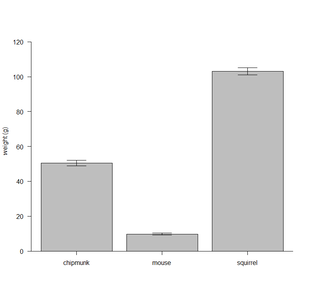
|
Great! It seems like that worked.
You can download the code for these functions and their example usage (including the 'animal weight' data) here:
You can download the code for these functions and their example usage (including the 'animal weight' data) here:
| summarytable___basicboxplot_functions.r |