Basic Mapping in R: Using R as a GIS
Spatial analyses, in many regards, can be done easier using R than a more classic GIS with a GUI (graphical user interface) like ArcGIS or qGIS. In this tutorial, I'll show how to make a basic map of two tree species (American sycamore and loblolly pine) using R and freely-available data sources. I'll also show how to plot points and overlay them as a spatial object.
Before progressing too far, here's the data used in this tutorial:
| ||||
Ok, so, to begin, let's first load our necessary packages:
library(raster); library(rgdal); library(dplyr); library(yarrr)
Note: You may have to install each of these with the function: install.packages("packagename") replacing 'packagename' with the name of the package to be downloaded. This MUST be in quotes for it to install.
As for these packages:
raster and rgdal are both important for doing a lot of basic spatial tasks in R. For example, rgdal has a great function (readOGR()) for reading vector shapefiles (like a polygon you might get from ArcGIS; extension = .shp). raster, likewise, has many functions for processing spatial data (both vector and raster files, despite the name). dplyr is useful for processing/handling data of many types and yarrr is a nice package for overlaying shapes with plot() with partial color transparency
####################################
Next, I like to save a few 'crs' that I'll use later. "CRS" stands for 'coordinate reference system' and you can think of this as your coordinate system (projected or geographic). I'll show you two different formats here for an UNprojected (geographic) crs (NAD83 lat/long) and a projected crs (Alber's Equal Area projection). I'll save each as an R object that we can use later (though you could also paste them into a function as-is; I just think this looks cleaner):
# saving projections/datums for later use
LongLatCRS <-'+init=epsg:4326'
albersCRS <- '+proj=aea +lat_1=20 +lat_2=60 +lat_0=40 +lon_0=-96 +x_0=0 +y_0=0 +ellps=GRS80'
Ok! Let's now try reading in a vector shapefile of the entire US. We will do this using the readOGR function from rgdal. Then, let's check the class() of this object (we want it to be a spatial polygons dataframe; 'sp'). Finally, let's check the coordinate reference system of this object using crs():
# read in US states shapefile
b0 <- rgdal::readOGR("D:\\Desktop Files November 2019\\fireflies\\us state bounds\\us_states\\us_states.shp")
class(b0) # sp
crs(b1) # CRS arguments: +proj=longlat +datum=WGS84 +no_def
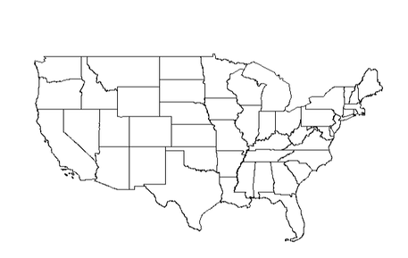
Ok things look good with our object "b0" -- let's take a look by plotting with the plot() function:
plot(b0)

Ok! That seems to have worked! However, we have a very expansive map. Let's try and subset this a bit so we are using only the continental US -- we can do this by removing the extra land units using bracket notation:
# subsetting so we just have the continental US
b1 <- b0[b0$name != 'Alaska',]
b1 <- b1[b1$name != 'Hawaii',]
b1 <- b1[b1$name != 'Guam',]
b1 <- b1[b1$name != 'Northern Mariana Islands',]
b1 <- b1[b1$name != 'American Samoa',]
b1 <- b1[b1$name != 'United States Virgin Islands',]
b1 <- b1[b1$name != 'Puerto Rico',]
# plot
plot(b1) # looks nice
Ok this looks great! Now let's bring in a shapefile of the great lakes and overlay it using the same procedure.
Below, we do four things:
First, we read in the shapefile using readOGR()
Second, we check the class of the object using class()
Third, we transform the gl0 object using spTransform() to make sure its crs = lat/long (the same as with the US states)
Fourth, we plot() -- note the: add = TRUE -- this makes sure our new object is added to the existing map
The third step here is critical because we need the crs of objects to overlap with each other. If you're having problems getting objects to overlay like this, a helpful first step is to check the extent of an object using extent(gl0) to see the spatial extent.
gl0 <- rgdal::readOGR("D:\\Working Files\\Main Storage\\ArcGIS\\Vector Shapefiles\\Great_Lakes (1)\\Great_Lakes.shp")
class(gl0) # sp
gl1 <- spTransform(gl0, CRS(LongLatCRS)) # transform
plot(gl1, add = TRUE, col = "lightblue")
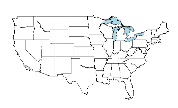
Ok! The map of the US with the great lakes overlaid looks good. Now let's bring in some tree range maps.
I'm by no means an expert with free spatial data, however, the digital range maps from the US Forest Service by E. L. Little seem pretty useful. They can be downloaded here:
https://www.fs.fed.us/nrs/atlas/littlefia/species_table.html
With this in mind, there's one tricky aspect to using this dataset; when you read in the file and check the CRS, R returns an "NA" because the crs is undefined. The Little trees dataset has the following information (here) about the crs of these data. I'd never built a +proj4 string before, however, this site has useful information on interpreting them.
All in all, I found this projection was exactly what we need for the dataset -- I'll spare you the details.
LittleProjection <- '+proj=aea +lat_1=38 +lat_2=42 +lat_0=40 +lon_0=-82 +x_0=0 +y_0=0 +ellps=GRS80 +datum=NAD27 +units=m +no_defs'
Now that we have that, let's read in the shapefile (using readOGR()) for the American sycamore and assign it the new crs (crs()). Then, let's transform the data to match the us states and great lakes objects, above using spTransform(). Finally, let's plot the range over our US states using plot().
amsyc0 <- rgdal::readOGR("C:\\Users\\obses\\Desktop\\sycamore\\litt731av.shp")
crs(amsyc0) <- LittleProjection
amsyc1 <- spTransform(amsyc0, LongLatCRS) # transform
plot(b1)
plot(amsyc1, add = TRUE, col = yarrr::transparent(orig.col = "cornflowerblue", trans.val = 0.65, maxColorValue = 255))
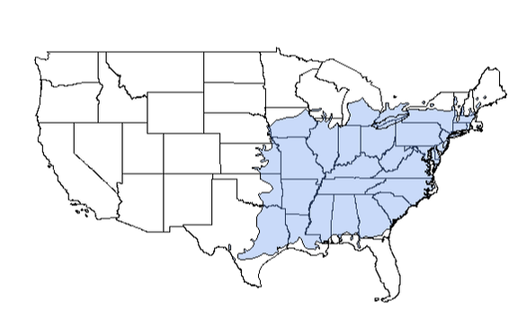
Great!
That looks good. Now let's do the same procedure for loblolly pine.
That looks good. Now let's do the same procedure for loblolly pine.
lobpin0 <- rgdal::readOGR("C:\\Users\\obses\\Desktop\\loblolly\\litt131av.shp") # read shapefile
crs(lobpin0) <- LittleProjection # define projection
lobpin1 <- spTransform(lobpin0, LongLatCRS) # transform
plot(lobpin1, add = TRUE, col = yarrr::transparent(orig.col = "yellow", trans.val = 0.65, maxColorValue = 255))
plot(gl1, add = TRUE, col = "lightblue")
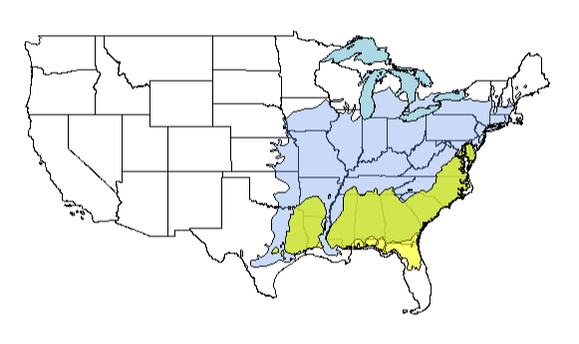
Looking good!
However, there's one aspect I don't really like; I was hoping to overlay BLUE and YELLOW to get an overlapping area of green. It didn't work all that well, as you can see. So, as an alternative, I can calculate the intersection of these two vector files, plot this object overtop everything and color it green.
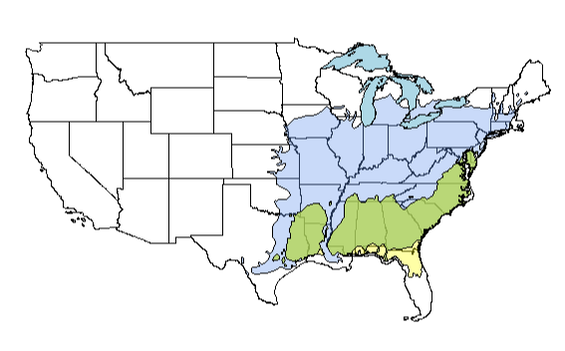
To calculate the intersection, I use intersect() with the two vector files for the trees (I had to specify raster:: to keep R from getting confused). Then simply plot the new object (clip1) overtop everything:
However, there's one aspect I don't really like; I was hoping to overlay BLUE and YELLOW to get an overlapping area of green. It didn't work all that well, as you can see. So, as an alternative, I can calculate the intersection of these two vector files, plot this object overtop everything and color it green.
To calculate the intersection, I use intersect() with the two vector files for the trees (I had to specify raster:: to keep R from getting confused). Then simply plot the new object (clip1) overtop everything:
clip1 <- raster::intersect(amsyc1, lobpin1)
plot(clip1, add = TRUE, col = yarrr::transparent(orig.col = "darkolivegreen3", trans.val = 0.4, maxColorValue = 255))
Ok! That basically concludes this tutorial; the last component remaining is to export any shapefiles from this exercise. Doing so can be useful if you want to do mapping in another GIS (e.g., I like qGIS) or perhaps send shapefiles to a collaborator. You can do this using the writeOGR() command; see example below:
writeOGR(b1, "C:\\Users\\obses\\Desktop\\forcody\\us_states.shp", driver="ESRI Shapefile", layer='test') # us_states
Finally, here's all of the R code for this exercise:
| ||||