Hierarchical Distance Models
Hierarchical distance models (HDM) are a relatively new type of model that can be implemented in unmarked. They are a valuable tool because, like classic distance models, HDMs estimate density of animals using observed distances and single surveys to assess- and account for detection probability.
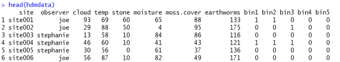
To begin, you should ensure that your data are formatted properly; in this worked example, we will use this fake dataset:
| ||||
Some things to notice: first, each ROW is a site visit. Each column represents the metadata for the site - both survey covariates (e.g., observer name, cloud cover) and site covariates (e.g., moss cover, earthworm [prey] abundance, etc.). The last thing to notice is that there are distance bins - in this case, bins 1-5. These bins represent the distance data. The count within each bin represents the number of animals detected in each distance bin. So, at site001, Joe observed one animal in the first bin (let's say, 0-1 m from the transect) and one animal in the second bin (1-2 m from the transect). Likewise, At site004, Stephanie observed one animal in the first bin, one animal in the second bin, and one in the third bin. These data need not be 1/0, this subset of data are just coincidentally that way. If Stephanie had seen all three animals in the same distance bin instead of spread across all three, the distance data for that site would be 3-0-0-0-0.
Ok, now that we are familiar with the dataset, let's begin the analysis itself. Begin by loading the needed packages (unmarked and AICcmodavg):
library(unmarked)
library(AICcmodavg)
Next, of course, you will want to set your working directory ('setwd') and import the .csv ('read.csv'). You can set your working directory easily by copying the address of your file location from your file explorer, pasting it into R, and then replacing the single slashes (\) with double slashes (\\):
setwd("C:\\Users\\DJ\\Desktop")
data1<-read.csv("hdm_data_practice.csv", header=TRUE)
Like most unmarked analyses (and an increasing number of analyses in R, generally), you must begin by making an 'object' specific to the package. Think of this like an .INP file if you are familiar with programs like MARK. Before making an unmarked object (in this case, an unmarked dataframe for gdistsamp(), it's necessary/more convenient to create a few smaller objects first:
Observation data - creating an object now called 'observations1' makes the unmarkedFrame a bit less clunky.
breaks - this is the number of distance classes you have + 0; for example, if you have 0-1m, 1-2m, and 2-3m, you would have 4 breaks.
transect length - this should be the length of your distance transect, in meters.
site covariates - this includes your "site" and "survey" covariates together. This is a fairly poorly-named item but it is consistent with the poorly-named argument needed for unmarkedFrameGDS (see below).
sitecovs1[,"area"]<-((800*1000)/10000) - this piece of code (taken from Kery and Royle 2015) allows the model to predict output using ha.
observations1<-as.matrix(data1[,9:13]) # detection data
breaks<-c(0,1,2,3,4,5) # this needs to be length = J + 1 (J= no. of distance classes)
transect.length<-70
sitecovs1<-data1[,2:8] # both site covs and detection covs
sitecovs1[,"area"]<-((800*1000)/10000) # adds area in ha surveyed
Next, combine these into an unmarked frame using the objects we just created:
umf1 <- unmarkedFrameGDS(y = observations1, survey="line", unitsIn="m", siteCovs=sitecovs1,
dist.breaks=breaks, tlength=rep(transect.length, nrow(data1)),
numPrimary=1)
Great! If there was no warning message, it worked.
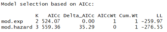
Nest you must assess which key function fits the dataset best. This function is fit to the data to serve as a model for how detection probability varies as a function of distance from the transect line - a critical component of distance models. Here I assess only two models: one for the hazard rate function (first) and another for the exponential key function (second). Note that you could assess a variety of others also included within gdistsamp.
Nest you must assess which key function fits the dataset best. This function is fit to the data to serve as a model for how detection probability varies as a function of distance from the transect line - a critical component of distance models. Here I assess only two models: one for the hazard rate function (first) and another for the exponential key function (second). Note that you could assess a variety of others also included within gdistsamp.
mod.hazard<-gdistsamp(~1,~1,~1, data=umf1, output="density", mixture="P", keyfun = "hazard")
mod.exp<-gdistsamp(~1,~1,~1, data=umf1, output="density", mixture="P", keyfun = "exp")
Note: I frequently get the following warning, often repeated several dozen times:
In log(cp[J + 1]) : NaNs produced
According to Kery and Royle (2015), this warning is totally normal and should essentially be ignored.
Now, let's create a list that includes only these two models and assess model fit (using the AIC ranking guidelines of Burnham and Anderson 2002) using aictab():
In log(cp[J + 1]) : NaNs produced
According to Kery and Royle (2015), this warning is totally normal and should essentially be ignored.
Now, let's create a list that includes only these two models and assess model fit (using the AIC ranking guidelines of Burnham and Anderson 2002) using aictab():
modlist1<-list(mod.hazard=mod.hazard, mod.exp=mod.exp)
aictab(modlist1)
And here is the ranked model set:
|
This suggests that the exponential key function model is MUCH better than the hazard rate model. Given this, we should use this function in all following models.
Next, let's evaluate detection probability. We have three detection covariates:
1) observer: a category for which surveyor conducted the survey (Joe, Becky, or Stephanie)
2) cloud cover: percent cloud cover at the start of the survey
3) temperature: temperature at the start of the survey
We can run each of these models for p (the third argument in the function) as well as a null model. Below is shown the creation of each model followed by ranking using the aictab() function:
p.null<-gdistsamp(~1,~1,~1, data=umf1, output="density", mixture="P", keyfun = "exp")
p.observer<-gdistsamp(~1,~1,~observer, data=umf1, output="density", mixture="P", keyfun = "exp")
p.cloud<-gdistsamp(~1,~1,~cloud, data=umf1, output="density", mixture="P", keyfun = "exp")
p.temp<-gdistsamp(~1,~1,~temp, data=umf1, output="density", mixture="P", keyfun = "exp")
modlist2=list(p.null=p.null, p.temp=p.temp, p.cloud=p.cloud, p.observer=p.observer)
aictab(modlist2)
And here is the ranked model set:
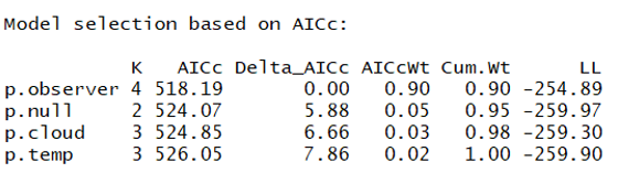
|
This suggests a pretty strong effect of observer on detection probability - this means that surveyors were unequal in their capacity to observe animals along the transect. Let's create a graph to visualize how our three surveyors did at detecting the organisms (disclaimer: there is likely a more efficient way to graph this but this method works):
newdat1<-cbind.data.frame(data1$site,data1$observer)
colnames(newdat1)<-c("site","observer")
p1<-getP(p.observer)
newdat1<-cbind(newdat1,p1)
colnames(newdat1)<-c("pointid","observer", "bin1", "bin2", "bin3", "bin4", "bin5")
joedata<- subset(newdat1, observer=="joe")
joep<-as.data.frame(c((max(joedata$bin1)),(max(joedata$bin2)),(max(joedata$bin3)),(max(joedata$bin4)),(max(joedata$bin5))))
joep<-cbind.data.frame(joep,"joe",c(1,2,3,4,5))
colnames(joep)<-c("p", "obs", "dist")
stephaniedata<- subset(newdat1, observer=="stephanie")
stephaniep<-as.data.frame(c((max(stephaniedata$bin1)),(max(stephaniedata$bin2)),(max(stephaniedata$bin3)),(max(stephaniedata$bin4)),(max(stephaniedata$bin5))))
stephaniep<-cbind.data.frame(stephaniep,"stephanie",c(1,2,3,4,5))
colnames(stephaniep)<-c("p", "obs", "dist")
beckydata<-subset(newdat1, observer=="becky")
beckyp<-as.data.frame(c((max(beckydata$bin1)),(max(beckydata$bin2)),(max(beckydata$bin3)),(max(beckydata$bin4)),(max(beckydata$bin5))))
beckyp<-cbind.data.frame(beckyp,"becky",c(1,2,3,4,5))
colnames(beckyp)<-c("p", "obs", "dist")
plot(-10,-10, xlim=c(1,5), ylim=c(0,0.2), xlab="Distance from Observer (m)",
ylab="Detection Probability (p)")
lines(stephaniep$dist,stephaniep$p, lty=1, col="blue")
lines(beckyp$dist,beckyp$p, lty=1, col="red")
lines(joep$dist,joep$p, lty=1, col="green")
text(3.5, 0.175, "Joe", col="green")
text(3.5, 0.160, "Becky", col="red")
text(3.5, 0.145, "Stephanie", col="blue")
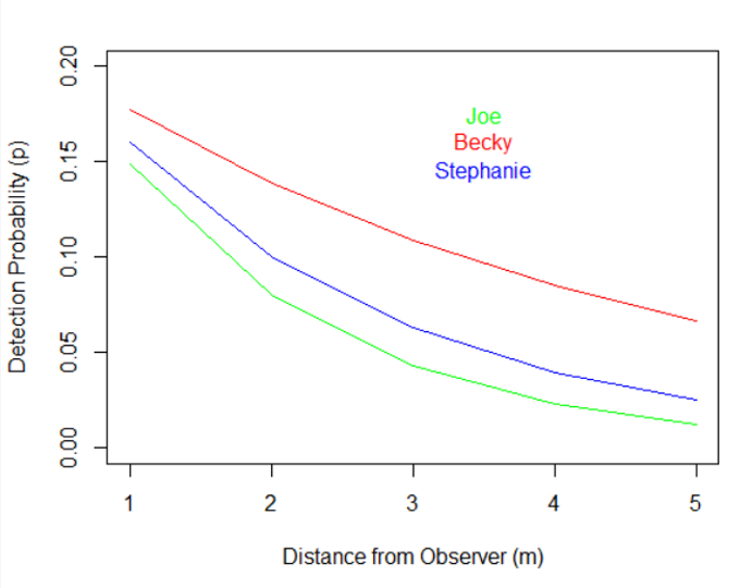
And this is the final graphical result:
|
As we can see from this graph, all observers had a more difficult time detecting the focal organisms as they were further from the transect line, but Becky was clearly the best. To put this into perspective, Becky was as likely to detect the organism when it was 5 m from the transect as Joe was when it was only 2 m away!
Great, now that we know that observer needs to be considered, we can use this as a detection covariate in all following models.
Now we model abundance (density; lambda) much in the same way we did above for detection probability. Note that the first argument is our abundance parameter. Below is shown a model set that includes a null model (which is actually the top-ranked detection model) as well as single-covariate models for habitat assessing the effects of:
stone - a stone cover metric around each transect
moisture - a moisture content metric around each transect
moss - a moss cover metric around each transect
earthworms - a metric of prey availability (count of worms) around each transect
Also below is code to rank the candidate model set using aictab(), as before:
lambda.null<-gdistsamp(~1,~1,~observer, data=umf1, output="density", mixture="P", keyfun = "exp")
lambda.stone<-gdistsamp(~stone,~1,~observer, data=umf1, output="density", mixture="P", keyfun = "exp")
lambda.moisture<-gdistsamp(~moisture,~1,~observer, data=umf1, output="density", mixture="P", keyfun = "exp")
lambda.mosscover<-gdistsamp(~moss.cover,~1,~observer, data=umf1, output="density", mixture="P", keyfun = "exp")
lambda.earthworms<-gdistsamp(~earthworms,~1,~observer, data=umf1, output="density", mixture="P", keyfun = "exp")
modlistb=list(lambda.null=lambda.null, lambda.stone=lambda.stone, lambda.moisture=lambda.moisture,
lambda.mosscover=lambda.mosscover, lambda.earthworms=lambda.earthworms)
aictab(modlistb)
And here is the resulting model ranking:
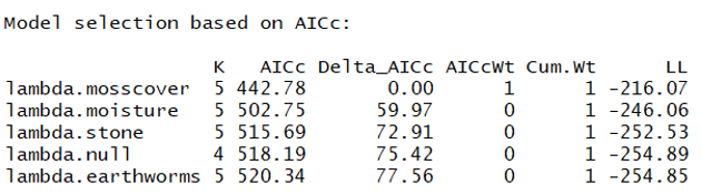
|
Great - this suggests that moss cover is a much better model than the null. The same is true for moisture and stone cover. In fact, the only predictor that does a worse job explaining the abundance of our organism is the earthworm covariate.
Let's visualize one of these relationships. Below is the code to predict the density of the focal taxa using moss cover as an explanatory variable (with 95%CIs):
Let's visualize one of these relationships. Below is the code to predict the density of the focal taxa using moss cover as an explanatory variable (with 95%CIs):
newdat<-data.frame(moss.cover=seq(min(data1$moss.cover), max(data1$moss.cover), length.out = 100))
expectedN<-predict(lambda.mosscover, type="lambda", newdata=newdat, appendData=TRUE)
print(expectedN)
plot(1, xlim=c(0,100), ylim=c(0,200), type="n", axes=T, xlab="Moss cover (%)", pch=20, ylab="Animal Density (ind./ha)", family="serif", cex.lab=1.25, cex.main=1.75)
lines(expectedN$moss.cover, expectedN$Predicted, col="black", lwd=2)
lines(expectedN$moss.cover, expectedN$lower, lty=2, col="black")
lines(expectedN$moss.cover, expectedN$upper, lty=2, col="black")
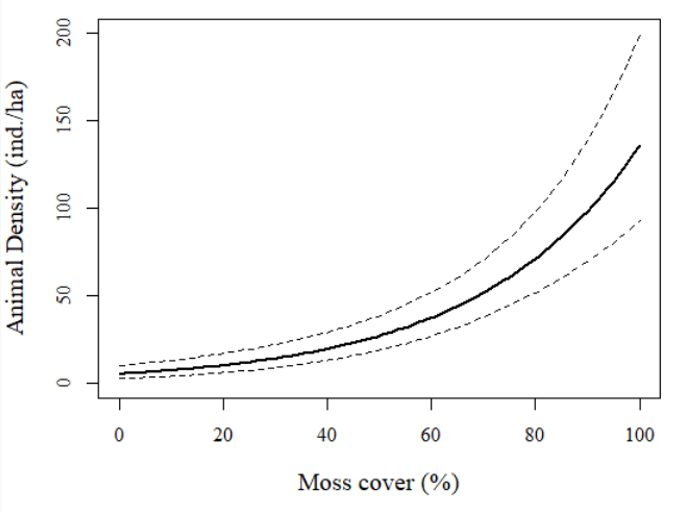
And here is the graphical output:
|
Fantastic! We can see a very strong pattern of abundance associated with moss cover. Sites with < 50% moss cover generally had fewer than 25 animals/ha or so while sites with 100% moss cover had >125 animals/ha (or even as many as 200/ha based on the upper 95%CI!). Very cool stuff.
As with the posts before on occupancy models, this post really just 'scratches the surface' of hierarchical distance modeling but this should 'get your feet wet' for those totally new to hierarchical distance models in unmarked. Feel free to email me if you have any questions on the content of this tutorial and feel free to share with those interested! Oh, and definitely check out our 2018 bumblebee paper that uses this exact method on forest Bombus spp.!
As with the posts before on occupancy models, this post really just 'scratches the surface' of hierarchical distance modeling but this should 'get your feet wet' for those totally new to hierarchical distance models in unmarked. Feel free to email me if you have any questions on the content of this tutorial and feel free to share with those interested! Oh, and definitely check out our 2018 bumblebee paper that uses this exact method on forest Bombus spp.!