Single-season Occupancy Models
Occupancy models have been for a staple of wildlife studies for nearly two decades now. Since the publication of MacKenzie et al. (2005): Occupancy Estimation and Modeling, use of occupancy analysis in ecological study has rapidly proliferated. More recently, occupancy models were developed for use in unmarked in R which has made them more available yet (see Kery and Royle 2015: Applied Hierarchical Modeling in Ecology for a great primer). Here I walk you through a simple example of a single-season occupancy analysis using some fake data for a fake organism in fake habitat. Begin by downloading the dataset:
| |||
Let's begin by loading the needed packages (unmarked and AICcmodavg):
library(unmarked)
library(AICcmodavg)
Next, of course, you will want to set your working directory ('setwd') and import the .csv ('read.csv'). You can set your working directory easily by copying the address of your file location from your file explorer, pasting it into R, and then replacing the single slashes (\) with double slashes (\\):
setwd("C:\\Users\\DJ\\Desktop")
data1<-read.csv("occu_data_practice.csv", header=TRUE)
Once you've imported the data (called 'data1'), we must create an 'unmarked frame'. This data object is that used by unmarked for analysis. Note that the unmarked frame has three main parts:
1) "y" (the occupancy data),
2) "siteCovs" (covariates which are site specific... like grass cover and sapling cover),
3) "obsCovs" (covariates which are observation-specific... like time since sunrise (tssr) and wind). These change during each visit to a single site. Note that we have two visits/season so we therefore have two objects within "y" (each survey for the organism) and two objects for each of our "obsCovs" (e.g., wind during each survey) but only ONE for each of our "siteCovs"... these things remain the same during each survey (e.g., canopy cover doesn't change, no matter how many times you visit).
umf <-unmarkedFrameOccu(
y=data1[,c('det1','det2')],
siteCovs=data1[,c('ha','canopy','sapling','shrub','forb','fern','grass','moss','litter')],
obsCovs=list(sky=data1[,c('cloud1','cloud2')], tssr=data1[,c('time1','time2')],
wind=data1[,c('wind1', 'wind2')], date=data1[,c('date1','date2')]))
Time to create some occupancy models! The model function ("occu") has three main arguments:
~"p", ~"psi", and "data". "p" is shorthand for detection probability. If you want to keep it constant, place a 1 here. "psi" is shorthand for occupancy. It can be held constant in the same way. "data" should be your unmarked frame. Below I create single-covariate occupancy models for detection probability but keep occupancy constant (we will get to that next). I also created a null model called "p.null" which includes no covariates for p or psi.
~"p", ~"psi", and "data". "p" is shorthand for detection probability. If you want to keep it constant, place a 1 here. "psi" is shorthand for occupancy. It can be held constant in the same way. "data" should be your unmarked frame. Below I create single-covariate occupancy models for detection probability but keep occupancy constant (we will get to that next). I also created a null model called "p.null" which includes no covariates for p or psi.
p.null<-occu(~1~1, data=umf)
p.wind<-occu(~wind~1, data=umf)
p.sky<-occu(~sky~1, data=umf)
p.date<-occu(~date~1, data=umf)
p.time<-occu(~tssr~1, data=umf)
Once those models are run, I usually create a list containing each model and then use the aictab() function to rank the models in descending order of AIC and create a table. This function is really quite handy.
modlist1<-list(
p.null=p.null, p.wind=p.wind,
p.sky=p.sky,p.time=p.time, p.date=p.date)
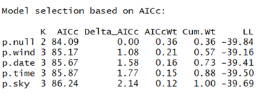
aictab(modlist1)
And here is the ranked model set:
|
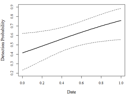
Ok so it looks like nothing we examined here impacts detection probability. Why do I say that? In this case it is clear: the null model (which contains no covariates for detection) is the top-ranked model. In essence, the most parsimonious explanation for what describes detection is: nothing (given the covariates we considered, anyway). This means that for a covariate like, say, cloud cover, there should be no relationship with detection probability. Let's visualize this by predicting detection probability using the cloud cover model (we expect a flat line):
newsky<-data.frame(sky=seq(0, 100, length.out=100))
pred.p<-predict(p.sky, type="det", newdata=newsky)
plot(1, xlim=c(0,100), ylim=c(0,1), type="n", axes=T, xlab="Sky Condition (% Cloud Cov.)",
pch=20, ylab="Detection Probability", family="serif",
cex.lab=1.25, cex.main=1.75)
lines(newsky$sky, pred.p$Predicted, col="black", lwd=2)
lines(newsky$sky, pred.p$lower, lty=2, col="black")
lines(newsky$sky, pred.p$upper, lty=2, col="black")
|
Great! This makes good sense. Detection is basically a flat line around 0.75 suggesting that, regardless of cloud cover, we always have a probability of detecting the focal species of ~0.75 on each visit (which isn't bad!). We can also check beta coefficient 95% confidence intervals for the model of interest (overlapping zero would suggest a weak effect):
confint(p.sky, type="det")
Notice that the 95% confidence intervals for the cloud cover parameter overlap zero.
For the rest of this analysis, we will analyze as if cloud cover were, indeed, a useful covariate for demonstrative purposes. Recognize that we wouldn't normally do this for a covariate as uninformative as cloud cover (unless it were truly explanatory). Next we create occupancy models using "sky" to explain detection and each of our site covariates to explain occupancy - including a detection-only model ("psi.null") as our null model. We also create a list of models and rank them using the same function as above (aictab):
For the rest of this analysis, we will analyze as if cloud cover were, indeed, a useful covariate for demonstrative purposes. Recognize that we wouldn't normally do this for a covariate as uninformative as cloud cover (unless it were truly explanatory). Next we create occupancy models using "sky" to explain detection and each of our site covariates to explain occupancy - including a detection-only model ("psi.null") as our null model. We also create a list of models and rank them using the same function as above (aictab):
psi.null<-occu(~sky~1, data=umf)
psi.canopy<-occu(~sky~canopy, data=umf)
psi.sap<-occu(~sky~sapling, data=umf)
psi.shrub<-occu(~sky~shrub, data=umf)
psi.forb<-occu(~sky~forb, data=umf)
psi.fern<-occu(~sky~fern, data=umf)
psi.grass<-occu(~sky~grass, data=umf)
psi.moss<-occu(~sky~moss, data=umf)
modlist2<-list(
psi.null=psi.null, psi.canopy=psi.canopy, psi.sap=psi.sap,
psi.shrub=psi.shrub, psi.forb=psi.forb, psi.fern=psi.fern, psi.grass=psi.grass,
psi.moss=psi.moss)
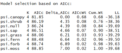
aictab(modlist2)
|
Based on this AIC table, it seems that canopy is an important predictor. The null model is > 2.0 from this model suggesting that it is not "competing" (in the words of Burnham and Anderson 2002). Let's check the confidence intervals on the beta coefficient for the canopy cover term in that psi.canopy model:
confint(psi.canopy, type="state")
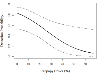
Non-overlapping with zero! That suggests the covariate is a strong predictor! Let's visualize this relationship using a graph of the predicted relationship based on that model and some 'fake data' (as we did with the detection example above):
newcan<-data.frame(canopy=seq(min(data1$canopy),max(data1$canopy), length.out=100))
pred.psi<-predict(psi.canopy, type="state", newdata=newcan)
plot(1, xlim=c(min(data1$canopy),max(data1$canopy)), ylim=c(0,1), type="n", axes=T, xlab="Canpopy Cover (%)",
pch=20, ylab="Detection Probability", family="serif",
cex.lab=1.25, cex.main=1.75)
lines(newcan$canopy, pred.psi$Predicted, col="black", lwd=2)
lines(newcan$canopy, pred.psi$lower, lty=2, col="black")
lines(newcan$canopy, pred.psi$upper, lty=2, col="black"
|
Very cool! It looks like there is a strong dropoff on occupancy from high occupancy (>0.80) at low canopy cover to very low occupancy (~0) when canopy cover is high.
This example, while just 'scratching the surface' of occupancy models should give you a nice introduction to their use. Feel free to email me if you have any questions on the content of this tutorial and feel free to share with those interested!
This example, while just 'scratching the surface' of occupancy models should give you a nice introduction to their use. Feel free to email me if you have any questions on the content of this tutorial and feel free to share with those interested!

