Preparing Data for Single-season Occupancy Models in R
As I describe on the page for single-season occupancy analyses (here), occupancy models have been a staple of wildlife conservation for decades. The development of the R package unmarked has brought this tool to the R interface has opened a number of important doors for occupancy modeling. In my experience implementing occupancy models in R, one of the most time-consuming components of data analysis is actually the data prep. In this post, I will provide an overview of one method of data prep for occupancy modeling in R using the dplyr package. Note that this method is by no means the most efficient one, however, provides a fairly straightforward path to data prep that is digestible for the novice codester (like myself).
Begin by downloading 'raw_survey_data'. Open the file and take careful note of the overall data structure - the file includes multiple rows for each survey event (or each visit to each site). Each row represents an observation of an organism during a single site visit event. If you observed 9 species of organism during a given visit, there should be 9 rows for that site's visit. Note that ALL site visits must be present within this file, even if no organisms were observed. This means that, for visits with both 1 species observation and 0 species observation, there should be 1 row in the dataset.
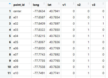
Also download the 'point_locations' file. This provides the coordinates for each site and we will link these site coordinates to the raw survey data for analysis.
Begin by downloading 'raw_survey_data'. Open the file and take careful note of the overall data structure - the file includes multiple rows for each survey event (or each visit to each site). Each row represents an observation of an organism during a single site visit event. If you observed 9 species of organism during a given visit, there should be 9 rows for that site's visit. Note that ALL site visits must be present within this file, even if no organisms were observed. This means that, for visits with both 1 species observation and 0 species observation, there should be 1 row in the dataset.
Also download the 'point_locations' file. This provides the coordinates for each site and we will link these site coordinates to the raw survey data for analysis.
|
| |||||
Let's begin by loading the needed packages (dplyr):
library(dplyr)
Next, of course, you will want to set your working directory ('setwd') and import the .csv ('read.csv') files for both the raw survey data (with fake frog data) and the site coordinates (which are centered around State College, Pennsylvania). You can set your working directory easily by copying the address of your file location from your file explorer, pasting it into R, and then replacing the single slashes (\) with double slashes (\\):
setwd("C:\\Users\\DJ\\Desktop\\fake_occu_data") #set working directory
frogs <- read.csv("raw_survey_data.csv") # read raw frog data into R
sitecoords1 <- read.csv("point_locations.csv") # read coordinate data into R
Next, it's probably worth taking the time to view the raw frog observation data
View(frogs)
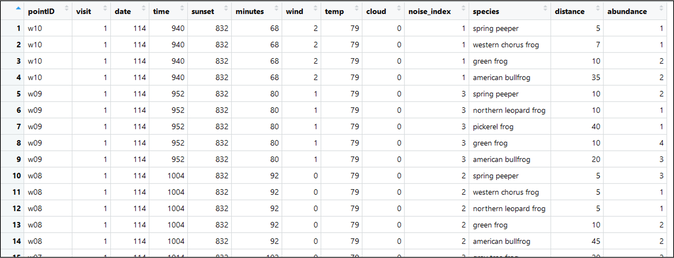
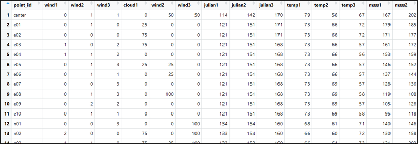
As you can see, the data include a unique point ID for each point location (the coordinates of which are stored in another file), a visit # (1, 2, or 3 for each visit to each site), a date (Julian or numerical), time of day, time of sunset (frog surveys occur after dark), "minutes" (which represents minutes since sunrise), "wind" which represents an index of how windy the site was during a given survey, "temp" in Fahrenheit, cloud cover, "noise_index" which represents an index of how noisy the site was during a given survey, frog species, distance (to nearest individual) and abundance (of each species).
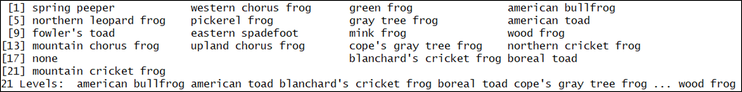
Let's view all the species to get a sense for the data contained in the file:
Let's view all the species to get a sense for the data contained in the file:
unique(frogs$species)
For our single season occupancy models, we will want to choose ONE species to model. We will get to that later.
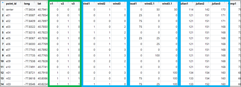
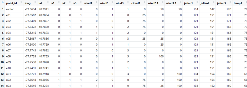
Now, recall that, for single-season occupancy models, we want our data structure to include a SINGLE row for each site with three columns for detections (e.g., 110, 000, 101, 111, etc.) and three columns for each of our detection variables. This data structure should look something like the following picture with our detection history highlighted in green and several survey covariate histories outlined in blue:
Now, recall that, for single-season occupancy models, we want our data structure to include a SINGLE row for each site with three columns for detections (e.g., 110, 000, 101, 111, etc.) and three columns for each of our detection variables. This data structure should look something like the following picture with our detection history highlighted in green and several survey covariate histories outlined in blue:
Preparing Survey Covariates
I break this down here in several chunks. First, we create the blue pieces -- the detection data file (because this is the most complicated -- let's get it out of the way first). Here's the method where I do this one visit at a time, then combine them all:
First, extract just the first visits to each site:
First, extract just the first visits to each site:
frogsV1 <- subset(frogs, visit == 1)
Then link the coordinate data with each site. This is effectively a left join where the components of 'sitecoords1' are used as a base since this is a file with one row for each site (our desired end goal).
lookup_1a <- merge(x = sitecoords1, by.x = "point_id", y = frogsV1, by.y = "pointID", all.x = TRUE) #vlookup
Then sites must be identified as a group - this does not change the APPEARANCE of the
file, however, is important for summarising ('summarise()') each visit's detection data:
file, however, is important for summarising ('summarise()') each visit's detection data:
lookup_1b <- group_by(lookup_1a, point_id)
Next, let's summarize the dataset for each detection covariate. Summarise gives you summary data for each group. In this case, you can choose anything -- all of the values are the same; you could choose min(), max(), or whatever - I chose mean() here. In any case, this bit of code gives you each detection covariate needed for occupancy modeling
lookup_1cloud <- data.frame(summarise(lookup_1b, cloud = mean(cloud)))
lookup_1julian <- data.frame(summarise(lookup_1b, julian = mean(date)))
lookup_1temp <- data.frame(summarise(lookup_1b, temp = mean(temp)))
lookup_1wind <- data.frame(summarise(lookup_1b, wind = mean(wind)))
lookup_1msss <- data.frame(summarise(lookup_1b, msss = mean(minutes)))
lookup_1noise <- data.frame(summarise(lookup_1b, noise = mean(noise_index))
Great!
Now do this again for visits 2 and 3 (shown below without detailed annotation):
Now do this again for visits 2 and 3 (shown below without detailed annotation):
# second visit
frogsV2 <- subset(frogs, visit == 2) # removing all data except from visit 2
lookup_2a <- merge(x = sitecoords1, by.x = "point_id", y = frogsV2, by.y = "pointID", all.x = TRUE) #vlookup
lookup_2b <- group_by(lookup_2a, point_id)
lookup_2cloud <- data.frame(summarise(lookup_2b, cloud = mean(cloud)))
lookup_2julian <- data.frame(summarise(lookup_2b, julian = mean(date)))
lookup_2temp <- data.frame(summarise(lookup_2b, temp = mean(temp)))
lookup_2wind <- data.frame(summarise(lookup_2b, wind = mean(wind)))
lookup_2msss <- data.frame(summarise(lookup_2b, msss = mean(minutes)))
lookup_2noise <- data.frame(summarise(lookup_2b, noise = mean(noise_index)))
# third visit
frogsV3 <- subset(frogs, visit == 3) # removing all data except from visit 3
lookup_3a <- merge(x = sitecoords1, by.x = "point_id", y = frogsV3, by.y = "pointID", all.x = TRUE) #vlookup
lookup_3b <- group_by(lookup_3a, point_id)
lookup_3cloud <- data.frame(summarise(lookup_3b, cloud = mean(cloud)))
lookup_3julian <- data.frame(summarise(lookup_3b, julian = mean(date)))
lookup_3temp <- data.frame(summarise(lookup_3b, temp = mean(temp)))
lookup_3wind <- data.frame(summarise(lookup_3b, wind = mean(wind)))
lookup_3msss <- data.frame(summarise(lookup_3b, msss = mean(msss)))
lookup_3noise <- data.frame(summarise(lookup_3b, noise = mean(noise_index)))
OK!
Getting closer. Now combining each visit's covariates of each type:
Getting closer. Now combining each visit's covariates of each type:
point_idVals <- data.frame("point_id" = lookup_1wind$point_id)
windVals <- cbind("wind1" = lookup_1wind$wind, "wind2" = lookup_2wind$wind, "wind3" = lookup_3wind$wind)
cloudVals <- cbind("cloud1" = lookup_1cloud$cloud, "wind2" = lookup_2cloud$cloud, "wind3" = lookup_3cloud$cloud)
julianVals <- cbind("julian1" = lookup_1julian$julian, "julian2" = lookup_2julian$julian, "julian3" = lookup_3julian$julian)
tempVals <- cbind("temp1" = lookup_1temp$temp, "temp2" = lookup_2temp$temp, "temp3" = lookup_3temp$temp)
msssVals <- cbind("msss1" = lookup_1msss$msss, "msss2" = lookup_2msss$msss, "msss3" = lookup_3msss$msss)
noiseVals <- cbind("noise1" = lookup_1noise$noise, "noise2" = lookup_2noise$noise, "noise3" = lookup_3noise$noise)
... and finally, combine into a single file:
AllDetCovs <- cbind(point_idVals, windVals, cloudVals, julianVals, tempVals, msssVals, noiseVals)
View(AllDetCovs)
Preparing Detection History
OK now that we finished that, we can prepare and add our detection history for a focal species. Let's select the wood frog (Lithobates sylvaticus) as our focal species and remove detections that occurred beyond 100 m from the observer:
frogs100 <- subset(frogs, distance <= 100) # removing detections beyond 100m
focalspecies <- "wood frog"
frogsV1 <- subset(frogs100, visit == 1) # removing all data except from visit 1
frogsV2 <- subset(frogs100, visit == 2) # removing all data except from visit 2
frogsV3 <- subset(frogs100, visit == 3) # removing all data except from visit 3
frogsV1_foc <- subset(frogsV1, species == focalspecies)
# subsetting focal species from first visit
frogsV2_foc <- subset(frogsV2, species == focalspecies)
# subsetting focal species from second visit
frogsV3_foc <- subset(frogsV3, species == focalspecies)
# subsetting focal species from third visit
Now to extract the occupancy data from visit 1:
# first visit
lookup1 <- merge(x = sitecoords1, by.x = "point_id", y = frogsV1_foc, by.y = "pointID", all.x = TRUE) #vlookup
lookup1$abundance[is.na(lookup1$abundance)] <- 0 # convert non-detections to zero in 'abundance'1
lookup1 <- mutate(lookup1, vis1 = if_else(abundance == 0, 0, 1))
visit1data <- data.frame("v1" = lookup1$vis1, "point1" = lookup1$point_id)
# point id added as a double-check
Now for visit 2 and visit 3
# second visit
lookup2 <- merge(x = sitecoords1, by.x = "point_id", y = frogsV2_foc, by.y = "pointID", all.x = TRUE) #vlookup
lookup2$abundance[is.na(lookup2$abundance)] <- 0
# convert non-detections to zero in 'abundance'
lookup2 <- mutate(lookup2, vis2 = if_else(abundance == 0, 0, 1))
visit2data <- data.frame("v2" = lookup2$vis2, "point2" = lookup1$point_id)
# point id added as a double-check
# third visit
lookup3 <- merge(x = sitecoords1, by.x = "point_id", y = frogsV3_foc, by.y = "pointID", all.x = TRUE) #vlookup
lookup3$abundance[is.na(lookup3$abundance)] <- 0
# convert non-detections to zero in 'abundance'
lookup3 <- mutate(lookup3, vis3 = if_else(abundance == 0, 0, 1))
visit3data <- data.frame("v3" = lookup3$vis3, "point3" = lookup1$point_id)
# point id added as a double-check
Now combine them together
# combining detection history
dethistory <- cbind(visit1data, visit2data, visit3data)
sitehistory <- merge(x = sitecoords1, by.x = "point_id", y = dethistory, by.y = "point1", all.x = TRUE) #vlookup
sitehistory <- select(sitehistory, -pointid, -point2, -point3) # delete trash columns
View(sitehistory)
|
Nearly done! Now combine into a single file:
FrogOccupancyData <- merge(x = sitehistory, by.x = "point_id", y = AllDetCovs, by.y = "point_id", all.x = TRUE) #vlookup
View(FrogOccupancyData)
Preparing Site Covariates
Okay. For this last piece, we will extract land cover characteristics from the National Land Cover Database (NLCD) that I have cropped to a buffer around the study area. First begin by downloading the NLCD raster file here:
| state_college_nlcd.tif |
And load the raster package so we can perform spatial analyses with it
library(raster)
A brief note about this file (like all raster files); the output will be numerical values for the categories of each land cover depicted by each cell. For example, you'll have a % for each category in its numerical form. This might look like: "41" (which represents deciduous forest) or "82" (which represents cultivated row crops). Click here to view the full NLCD legend.
Ok, first, let's pull the raster into R and reproject into Alber's Equal Area conic (a projection I regularly use):
Ok, first, let's pull the raster into R and reproject into Alber's Equal Area conic (a projection I regularly use):
nlcd_data <- raster(".\\state_college_nlcd.tif") # read raster
nlcd_data <- setMinMax(nlcd_data) # set extent of raster
# re-project the raster
nlcd_data_a <- projectRaster(from = nlcd_data, crs = "+proj=aea +lat_1=29.5 +lat_2=45.5 +lat_0=23 +lon_0=-96 +x_0=0+y_0=0 +ellps=GRS80 +datum=NAD83 +units=m +no_defs")
Note the LONG piece of text that reads: "+proj=aea +lat_1=29.5 +lat_2=45.5 +lat_0=23 +lon_0=-96 +x_0=0 +y_0=0 +ellps=GRS80 +datum=NAD83 +units=m +no_defs:"
Although this seems super crazy, this text is actually R's shorthand for Alber's Equal Area Conic projection. See here for more details.
Next, let's load in our coordinates, turn them into a spatial object, then reproject them into Alber's Equal Area Conic
Although this seems super crazy, this text is actually R's shorthand for Alber's Equal Area Conic projection. See here for more details.
Next, let's load in our coordinates, turn them into a spatial object, then reproject them into Alber's Equal Area Conic
coords1 <- data.frame(cbind("long" = sitehistory$long, "lat" = sitehistory$lat))
# read in coords of survey locs
sites1 <- sf::st_as_sf(coords1, coords = c("long", "lat"), crs = 4269) # turn the coords into a spatial object
# used crs = 4269 because this represents NAD83
sites1 <- sf::st_transform(sites1, crs = "+proj=aea +lat_1=29.5 +lat_2=45.5 +lat_0=23 +lon_0=-96 +x_0=0 +y_0=0 +ellps=GRS80 +datum=NAD83 +units=m +no_defs")
# reproject the points into the same as the raster
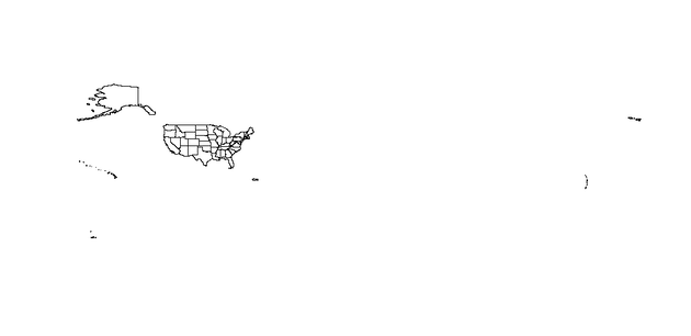
Now let's plot the data just to ensure that it worked properly:
plot(nlcd_data_a, xlim = c(xmin(nlcd_data_a) + 15000, xmax(nlcd_data_a) - 15000),
ylim = c(ymin(nlcd_data_a) + 10000, ymax(nlcd_data_a)))
plot(nlcd_data_a, add = TRUE)
plot(sites1, add = TRUE)
|
Great! Now let's extract the land cover within 500 m around each point from the underlying land cover.
extract1 <- raster::extract(x = nlcd_data_a, y = sites1, buffer = 500, df = TRUE)
extract1 <- data.frame(extract1)
Summarizing the data to be usable:
NLCD_freq <- mutate(extract1, NLCD = as.integer(state_college_nlcd)) %>%
group_by(ID, NLCD) %>%
summarise(freq = n()) %>%
ungroup() %>%
group_by(ID) %>%
mutate(ncells= sum(freq), prop_land = round(freq/ncells, 2) * 100) %>%
ungroup()
Re-assinging site names:
sitesPicklist <- data.frame(FalseName= seq(from = 1, to = 41, length.out = 41), OrigName = sitehistory$point_id)
Restructuring the dataset:
wide <- full_join(NLCD_freq, sitesPicklist, by=c("ID" = "FalseName")) %>%
dplyr::select(-ID, -freq, -ncells) %>%
tidyr::spread(NLCD, prop_land, fill = 0)
Finally, linking site data with detection data:
FinalData <- as.data.frame(full_join(wide, DetectionData, by = c("OrigName" = "point_id")))
View(FinalData)
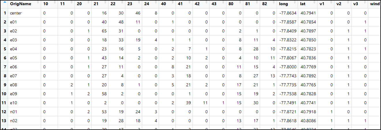
Fantastic! Our final data includes our percent landcover (10 - 82; the first dozen or so columns), siteID (OrigName), coordinates, a detection history for the wood frog, and detection covariates for each of our three visits. This is everything we need to conduct our occupancy analysis!
Download the R code for this tutorial here:
Download the R code for this tutorial here:
| frog_data_prep1.r |